Comprehensive Techniques for Solving Linear Equations

Understanding the Concept of Solving Linear Equations

What It Means to Solve Linear Equations

Solving linear equations involves determining the values of variables that satisfy the equation. Whether the equation contains one, two, or three variables, the goal is to find the specific values that make the equation true. These solutions represent the points or values where the equation balances perfectly.

Graphical Approach to Solving Linear Equations

Plotting and Interpreting Intersection Points

The graphical method involves drawing the lines represented by linear equations on a coordinate plane. The point where these lines intersect corresponds to the solution of the system. By selecting various values for one variable and calculating the corresponding values of the other, you can plot accurate points to form each line.

For instance, consider the system:

\[ 3x + 2y = 12 \]

\[ x - y = 2 \]

By choosing values for \( x \) and solving for \( y \), plot the points for both equations and identify their intersection.

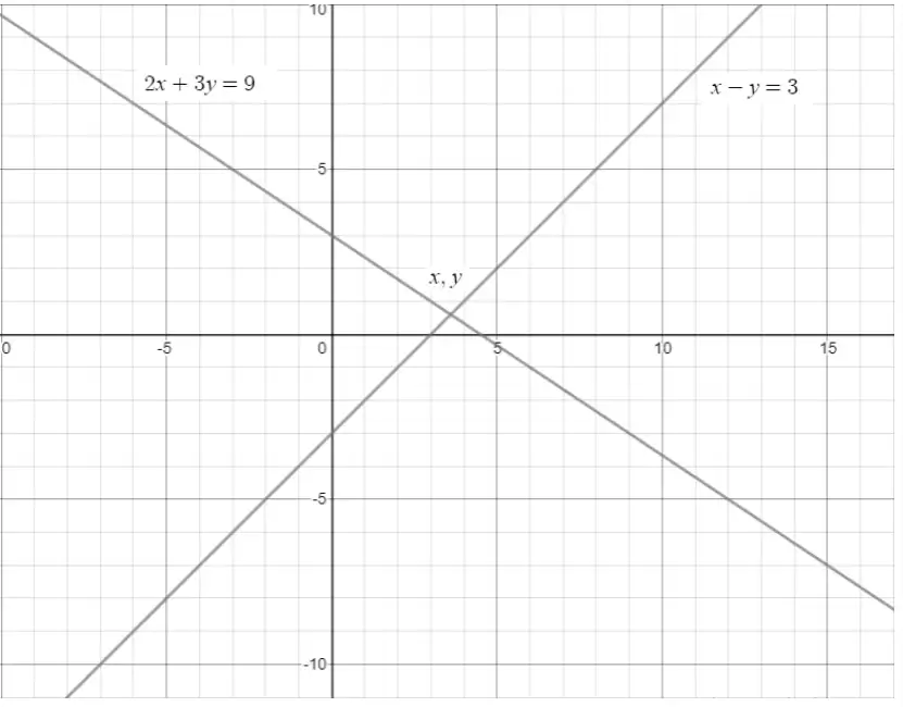
This image shows a graph with two straight lines. Each line represents a linear equation. The point where the two lines cross is the solution to the system of equations, meaning it satisfies both equations at the same time. Step-by-step explanation: 1. Each line on the graph is an equation with variables \(x\) and \(y\). 2. The equations shown are: \[ 2x + 3y = 9 \] and \[ x - y = 3 \] 3. To solve these equations graphically, we plot each line on the grid. 4. The solution to the system is where the two lines intersect. 5. From the graph, the intersection point is labeled as \((x, y)\), which gives the values of \(x\) and \(y\) that satisfy both equations.

Elimination Technique for Solving Linear Systems

Removing Variables to Simplify Equations

The elimination method focuses on removing one variable by making their coefficients equal and then subtracting or adding the equations. This reduces the system to a single-variable equation, which can be solved easily. After finding one variable, substitute it back to find the other.

Substitution Method for Finding Variable Values

Isolating and Replacing Variables

This method involves isolating one variable in one equation and substituting its expression into the other equation. This reduces the system to a single equation with one variable, which can be solved directly. Afterward, the found value is substituted back to find the remaining variable.

Cross Multiplication Method for Two-Variable Systems

Applying Cross Products to Solve Equations

The cross multiplication method uses a formula to directly calculate the values of variables in two-variable linear equations. It is especially useful when coefficients are known and can be substituted into the formula for quick solutions.

Given the system:

\[ a_1 x + b_1 y = c_1 \]

\[ a_2 x + b_2 y = c_2 \]

The solution is:

\[ x = \frac{b_1 c_2 - b_2 c_1}{a_1 b_2 - a_2 b_1}, \quad y = \frac{c_1 a_2 - c_2 a_1}{a_1 b_2 - a_2 b_1} \]

Matrix Approach to Solving Linear Equations

Using Matrices to Represent and Solve Systems

Matrix methods provide a structured way to solve linear equations, especially when dealing with multiple variables. The system is expressed as \( AX = B \), where \( A \) is the coefficient matrix, \( X \) is the variable matrix, and \( B \) is the constants matrix. The solution is found by calculating \( X = A^{-1} B \), where \( A^{-1} \) is the inverse of matrix \( A \).

This image shows a system of three linear equations written in matrix form. The goal is to solve for the variables \( x \), \( y \), and \( z \). Step-by-step explanation: 1. Write each equation with variables \( x \), \( y \), and \( z \) and their coefficients \( a_i \), \( b_i \), and \( c_i \). 2. Organize the coefficients into a 3x3 matrix on the left. 3. Place the variables in a column vector next to the coefficient matrix. 4. Put the constants \( d_1 \), \( d_2 \), and \( d_3 \) in a separate column vector on the right. 5. The matrix equation represents the system of equations as: \[ A \mathbf{x} = \mathbf{d} \] where \( A \) is the matrix of coefficients, \( \mathbf{x} \) is the variable vector, and \( \mathbf{d} \) is the constants vector. 6. To solve for \( \mathbf{x} \), you can use methods like matrix inversion or substitution.

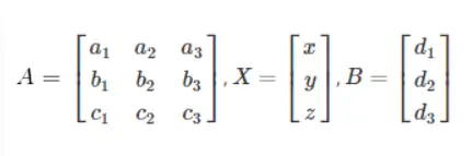
This image shows a matrix equation setup where \( A \) is a 3x3 matrix, \( X \) is a column vector with variables \( x, y, z \), and \( B \) is a column vector with constants \( d_1, d_2, d_3 \). Step-by-step explanation: 1. \( A \) is a matrix containing numbers or variables arranged in 3 rows and 3 columns. 2. \( X \) is a vector with 3 unknowns we want to find. 3. \( B \) is a vector with 3 known values. 4. The equation \( A \times X = B \) means when we multiply matrix \( A \) by vector \( X \), we get vector \( B \). 5. This is a system of 3 linear equations that can be solved to find the values of \( x, y, \) and \( z \).

Example: Solve the system:

\[ x + 2y = 5 \]

\[ 3x + 4y = 11 \]

Matrix form:

\[ A = \begin{bmatrix} 1 & 2 \\ 3 & 4 \end{bmatrix}, \quad X = \begin{bmatrix} x \\ y \end{bmatrix}, \quad B = \begin{bmatrix} 5 \\ 11 \end{bmatrix} \]

Calculate \( A^{-1} \):

\[ A^{-1} = \frac{1}{(1)(4) - (3)(2)} \begin{bmatrix} 4 & -2 \\ -3 & 1 \end{bmatrix} = \frac{1}{4 - 6} \begin{bmatrix} 4 & -2 \\ -3 & 1 \end{bmatrix} = \frac{1}{-2} \begin{bmatrix} 4 & -2 \\ -3 & 1 \end{bmatrix} \]

Multiply \( A^{-1} \) and \( B \):

\[ X = A^{-1} B = \frac{1}{-2} \begin{bmatrix} 4 & -2 \\ -3 & 1 \end{bmatrix} \begin{bmatrix} 5 \\ 11 \end{bmatrix} = \frac{1}{-2} \begin{bmatrix} (4)(5) + (-2)(11) \\ (-3)(5) + (1)(11) \end{bmatrix} = \frac{1}{-2} \begin{bmatrix} 20 - 22 \\ -15 + 11 \end{bmatrix} = \frac{1}{-2} \begin{bmatrix} -2 \\ -4 \end{bmatrix} \]

\[ X = \begin{bmatrix} 1 \\ 2 \end{bmatrix} \]

Therefore, \( x = 1 \) and \( y = 2 \).

Determinants and Cramer's Rule for Linear Systems

Utilizing Determinants to Find Variable Values

Cramer's Rule uses determinants to solve linear equations with two or three variables. It involves calculating the determinant of the coefficient matrix and replacing columns with the constants vector to find each variable's value.

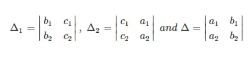
The image shows three determinants formed from the elements \( a_1, a_2, b_1, b_2, c_1, \) and \( c_2 \). The determinants are named \(\Delta_1\), \(\Delta_2\), and \(\Delta\). Step-by-step explanation: 1. A determinant is a special number calculated from a square matrix. 2. \(\Delta_1\) is the determinant of the 2x2 matrix with rows \((b_1, c_1)\) and \((b_2, c_2)\). 3. \(\Delta_2\) is the determinant of the 2x2 matrix with rows \((c_1, a_1)\) and \((c_2, a_2)\). 4. \(\Delta\) is the determinant of the 2x2 matrix with rows \((a_1, b_1)\) and \((a_2, b_2)\). 5. These determinants are used in solving systems of linear equations or finding areas in coordinate geometry.

The image shows a mathematical expression defining a determinant \(\Delta\) of a 3x3 matrix and three related determinants \(\Delta_1\), \(\Delta_2\), and \(\Delta_3\). Each \(\Delta_i\) is formed by replacing one column of the original matrix with a new column \(d_1, d_2, d_3\). Step-by-step explanation for high school students: 1. \(\Delta\) is a determinant of a 3x3 matrix with elements \(a_1, a_2, a_3\), \(b_1, b_2, b_3\), and \(c_1, c_2, c_3\). 2. \(\Delta_1\) is found by replacing the first column of the original matrix with the column \(d_1, d_2, d_3\), keeping the second and third columns the same. 3. \(\Delta_2\) replaces the second column with \(d_1, d_2, d_3\), keeping the first and third columns the same. 4. \(\Delta_3\) replaces the third column with \(d_1, d_2, d_3\), while the first and second columns remain unchanged. This method is often used in solving systems of linear equations using Cramer's rule.

Example: Solve the system:

\[ 2x + 3y = 8 \]

\[ 4x - y = 2 \]

Calculate determinant \( \Delta \):

\[ \Delta = \begin{vmatrix} 2 & 3 \\ 4 & -1 \end{vmatrix} = (2)(-1) - (4)(3) = -2 - 12 = -14 \]

Calculate \( \Delta_x \):

\[ \Delta_x = \begin{vmatrix} 8 & 3 \\ 2 & -1 \end{vmatrix} = (8)(-1) - (2)(3) = -8 - 6 = -14 \]

Calculate \( \Delta_y \):

\[ \Delta_y = \begin{vmatrix} 2 & 8 \\ 4 & 2 \end{vmatrix} = (2)(2) - (4)(8) = 4 - 32 = -28 \]

Find variables:

\[ x = \frac{\Delta_x}{\Delta} = \frac{-14}{-14} = 1 \]

\[ y = \frac{\Delta_y}{\Delta} = \frac{-28}{-14} = 2 \]

Thus, \( x = 1 \) and \( y = 2 \).

Solving Linear Equations with a Single Variable

Simple Steps for One-Variable Equations

Equations with only one variable are straightforward to solve. The process involves isolating the variable on one side by combining like terms and moving constants to the opposite side. Graphically, the solution corresponds to the point where the line crosses the axis.

Approaches for Two-Variable Linear Equations

Choosing the Best Method for Systems with Two Variables

For equations involving two variables, multiple methods such as graphical, elimination, substitution, cross multiplication, matrix, and determinant methods are applicable. The choice depends on the complexity and context of the problem.

Strategies for Systems with Three or More Variables

Efficient Methods for Complex Linear Systems

When dealing with three or more variables, graphical, elimination, and substitution methods become cumbersome. The cross multiplication method and matrix-based approaches, including Cramer's rule, are preferred for their efficiency and clarity in handling multiple variables.

Quick Reference: Summary of Methods for Solving Linear Equations

Glossary of Key Terms

Frequently Asked Questions

What defines a linear equation?

A linear equation is one where variables appear only to the first power and graph as straight lines.

Which method is best for solving two-variable linear equations?

Methods like substitution, elimination, and cross multiplication are effective for two-variable systems depending on the problem context.

How do matrices simplify solving multiple variable equations?

Matrices organize coefficients and constants, allowing the use of matrix operations like inversion to find solutions efficiently.

Can graphical methods be used for three-variable systems?

Graphical methods are impractical for three or more variables due to the difficulty of visualizing higher dimensions.

What is the role of determinants in solving linear equations?

Determinants help determine if a system has a unique solution and are used in Cramer's rule to find variable values.