Comprehensive Guide to Differential Equations
Fundamentals and Classification of Differential Equations
Understanding the Concept and Basic Definition
A differential equation is a mathematical statement that relates a function with its derivatives, representing how the function changes with respect to an independent variable. Typically, it involves one or more derivatives of a dependent variable with respect to an independent variable, capturing dynamic relationships in various scientific fields such as physics, biology, and engineering.
For instance, the equation
\[ \frac{dy}{dx} = 4x \]
expresses the rate of change of \( y \) with respect to \( x \) as a function of \( x \) itself.
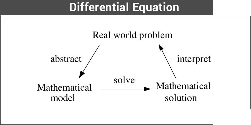
Visual representation of a differential equation
Example: Consider the differential equation \(\frac{dy}{dx} = 3x\). Here, the derivative of \( y \) with respect to \( x \) depends linearly on \( x \), demonstrating a simple first-order differential equation.
Order and Degree Explained
The order of a differential equation is determined by the highest derivative present in the equation. For example, the equation
\[ \frac{d^2y}{dx^2} + 3\frac{dy}{dx} + 2y = 0 \]
is a second-order differential equation because the highest derivative is the second derivative.
The degree refers to the power of the highest order derivative when the equation is expressed as a polynomial in derivatives. For example,
\[ \left(\frac{d^3y}{dx^3}\right)^2 + 5\frac{d^2y}{dx^2} = 0 \]
has degree 2 because the highest order derivative \(\frac{d^3y}{dx^3}\) is squared.
Example: Identify the order and degree of the equation \(\frac{dy}{dx} + \sin x = 0\).
Solution: The highest derivative is \(\frac{dy}{dx}\), which is first order, and it appears to the power 1, so the degree is 1.
Types of Differential Equations
Differential equations are broadly categorized based on their characteristics:
Ordinary Differential Equations (ODEs): Involve derivatives with respect to a single independent variable.
Partial Differential Equations (PDEs): Contain partial derivatives with respect to multiple independent variables.
Linear Differential Equations: The dependent variable and its derivatives appear linearly.
Nonlinear Differential Equations: Contain nonlinear terms of the dependent variable or its derivatives.
Homogeneous Equations: All terms are functions of the dependent variable and its derivatives only.
Nonhomogeneous Equations: Include terms independent of the dependent variable.
Methods for Solving Differential Equations
Separation of Variables Technique
This method applies when a differential equation can be expressed as a product of a function of the dependent variable and a function of the independent variable, such as
\[ \frac{dy}{dx} = f(y) \cdot g(x) \]
Rearranging, we get
\[ \frac{1}{f(y)} dy = g(x) dx \]
Integrating both sides yields the solution. This approach is straightforward for equations where variables can be separated cleanly.
Example: Solve \(\frac{dy}{dx} = y \sin x\).
Solution: Rewrite as \(\frac{1}{y} dy = \sin x dx\). Integrate both sides:
\[ \int \frac{1}{y} dy = \int \sin x dx \]
\[ \ln |y| = -\cos x + C \]
Therefore, the general solution is
\[ y = Ae^{-\cos x} \] where \(A = e^C\).
Integrating Factor Method
This technique is used for first-order linear differential equations of the form
\[ \frac{dy}{dx} + P(x) y = Q(x) \]
Multiplying both sides by the integrating factor
\[ \mu(x) = e^{\int P(x) dx} \]
transforms the equation into an exact derivative, allowing integration to find the solution.
Example: Solve \(\frac{dy}{dx} + 2y = e^{-x}\).
Solution: Here, \(P(x) = 2\), so integrating factor is
\[ \mu(x) = e^{\int 2 dx} = e^{2x} \]
Multiply both sides:
\[ e^{2x} \frac{dy}{dx} + 2 e^{2x} y = e^{2x} e^{-x} = e^{x} \]
Left side is derivative:
\[ \frac{d}{dx} \left( e^{2x} y \right) = e^{x} \]
Integrate both sides:
\[ e^{2x} y = \int e^{x} dx = e^{x} + C \]
Thus,
\[ y = e^{-x} + C e^{-2x} \]
Higher-Order Differential Equations
Equations involving derivatives of order two or higher are called higher-order differential equations. Their solutions often require specialized methods depending on the equation's form and linearity.
Applications and Real-Life Examples of Differential Equations
Practical Uses Across Various Fields
Differential equations are instrumental in modeling phenomena where quantities change continuously. Some key applications include:
Modeling population growth and radioactive decay through exponential functions.
Describing the cooling of objects, such as a hot beverage cooling to room temperature.
Analyzing electrical circuits and wave motion in physics.
Predicting the spread of diseases in epidemiology.
Optimizing investment strategies in economics.
Engineering applications like heat conduction and structural analysis.
Newton’s Law of Cooling: A Linear Differential Equation Example
Newton’s law states that the rate at which an object cools is proportional to the difference between its temperature and the ambient temperature. Mathematically, this is expressed as:
\[ \frac{dT}{dt} = -k (T - T_0) \]
where \(T\) is the temperature of the object at time \(t\), \(T_0\) is the surrounding temperature, and \(k\) is a positive constant.
Example: Suppose a cup of coffee at \(90^\circ \text{C}\) cools in a room at \(25^\circ \text{C}\). If the cooling constant is \(k = 0.1 \text{ min}^{-1}\), find the temperature after 10 minutes.
Solution: The differential equation is
\[ \frac{dT}{dt} = -0.1 (T - 25) \]
Rearranged:
\[ \frac{dT}{dt} + 0.1 T = 2.5 \]
The integrating factor is
\[ \mu(t) = e^{0.1 t} \]
Multiply both sides:
\[ e^{0.1 t} \frac{dT}{dt} + 0.1 e^{0.1 t} T = 2.5 e^{0.1 t} \]
Left side is derivative:
\[ \frac{d}{dt} \left( e^{0.1 t} T \right) = 2.5 e^{0.1 t} \]
Integrate:
\[ e^{0.1 t} T = 25 e^{0.1 t} + C \]
So,
\[ T = 25 + C e^{-0.1 t} \]
Using initial condition \(T(0) = 90\),
\[ 90 = 25 + C \implies C = 65 \]
Therefore,
\[ T(10) = 25 + 65 e^{-1} \approx 25 + 65 \times 0.3679 = 25 + 23.91 = 48.91^\circ \text{C} \]
Verification of a Solution to a Differential Equation
Consider the function \( y = e^{-2x} \). Verify if it satisfies the differential equation
\[ \frac{d^2 y}{dx^2} + 4 \frac{dy}{dx} + 4 y = 0 \]
Solution:
First derivative:
\[ \frac{dy}{dx} = -2 e^{-2x} \]
Second derivative:
\[ \frac{d^2 y}{dx^2} = 4 e^{-2x} \]
Substitute into the equation:
\[ 4 e^{-2x} + 4 (-2 e^{-2x}) + 4 e^{-2x} = 4 e^{-2x} - 8 e^{-2x} + 4 e^{-2x} = 0 \]
Since the left side equals zero, the function satisfies the differential equation.
Summary and Key Concepts
Concept | Description | Example |
|---|---|---|
Differential Equation | Equation involving derivatives of a function | \(\frac{dy}{dx} = 3x\) |
Order | Highest derivative order in the equation | Second order in \(\frac{d^2y}{dx^2} + y = 0\) |
Degree | Power of highest order derivative (if polynomial) | Degree 3 in \(\left(\frac{d^3y}{dx^3}\right)^3 + \cdots = 0\) |
Separation of Variables | Method to solve when variables can be separated | \(\frac{dy}{dx} = y \sin x\) |
Integrating Factor | Technique for first-order linear equations | \(\frac{dy}{dx} + 2y = e^{-x}\) |
Ordinary Differential Equation (ODE) | Involves derivatives with respect to one variable | \(\frac{dy}{dx} = f(x,y)\) |
Partial Differential Equation (PDE) | Involves partial derivatives with multiple variables | \(\frac{\partial u}{\partial t} = k \frac{\partial^2 u}{\partial x^2}\) |
Linear Equation | Dependent variable and derivatives appear linearly | \(\frac{dy}{dx} + P(x) y = Q(x)\) |
Nonlinear Equation | Contains nonlinear terms of dependent variable or derivatives | \(\frac{dy}{dx} = y^2 + x\) |
Newton’s Law of Cooling | Rate of cooling proportional to temperature difference | \(\frac{dT}{dt} = -k (T - T_0)\) |
Glossary of Key Terms
Term | Definition |
|---|---|
Differential Equation | An equation involving derivatives of a function with respect to one or more variables. |
Order | The highest derivative order present in a differential equation. |
Degree | The power of the highest order derivative when the equation is polynomial in derivatives. |
Dependent Variable | The function whose derivatives appear in the differential equation. |
Independent Variable | The variable with respect to which derivatives are taken. |
Separation of Variables | A method to solve differential equations by separating functions of different variables. |
Integrating Factor | A function used to simplify first-order linear differential equations for integration. |
Ordinary Differential Equation (ODE) | A differential equation involving derivatives with respect to a single variable. |
Partial Differential Equation (PDE) | A differential equation involving partial derivatives with respect to multiple variables. |
Newton’s Law of Cooling | A principle stating that the rate of temperature change is proportional to the difference from ambient temperature. |
Frequently Asked Questions
What is a differential equation?
A differential equation is a mathematical expression that relates a function to its derivatives, describing how the function changes with respect to one or more variables.
How are differential equations classified?
They are classified based on order, degree, linearity, and whether they involve ordinary or partial derivatives, such as ODEs and PDEs.
What does the order of a differential equation signify?
The order indicates the highest derivative present in the equation, determining the complexity of the solution.
Why are differential equations important?
They model dynamic systems in science and engineering, enabling prediction and understanding of natural and technological processes.
What are common methods to solve first-order differential equations?
Separation of variables and integrating factor methods are widely used to find solutions to first-order differential equations.