Understanding Bayes’ Theorem and Its Applications
Fundamentals of Bayes’ Theorem
Concept and Interpretation of Bayes’ Theorem
Bayes’ theorem provides a mathematical framework to calculate the probability of an event based on prior knowledge of related conditions. It is particularly useful when the probability of an event depends on the occurrence of another event, a concept known as conditional probability. Essentially, Bayes’ theorem allows us to update our beliefs about the likelihood of causes given observed outcomes.
For instance, consider three bags each containing balls of different colors: red, blue, and black. If we want to find the probability of selecting a blue ball from the second bag, knowing that a ball was drawn, Bayes’ theorem helps us incorporate this conditional information to find the correct probability.
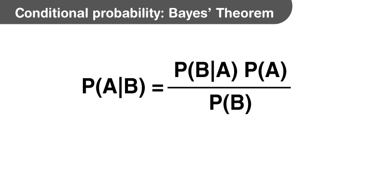
Visual representation of conditional probability
Example Problem
Suppose there are two bags: Bag A with 5 red and 5 black balls, and Bag B with 3 red and 7 black balls. A bag is chosen at random, and a black ball is drawn. What is the probability that the black ball came from Bag A?
Solution:
Let \( E_1 \) be the event of selecting Bag A, and \( E_2 \) be selecting Bag B. Let \( A \) be the event of drawing a black ball.
Since the bags are equally likely to be chosen,
\[ P(E_1) = P(E_2) = \frac{1}{2} \]
Probability of drawing a black ball from Bag A:
\[ P(A|E_1) = \frac{5}{10} = \frac{1}{2} \]
Probability of drawing a black ball from Bag B:
\[ P(A|E_2) = \frac{7}{10} \]
Using Bayes’ theorem, the probability that the black ball came from Bag A is:
\[ P(E_1|A) = \frac{P(E_1) P(A|E_1)}{P(E_1) P(A|E_1) + P(E_2) P(A|E_2)} = \frac{\frac{1}{2} \times \frac{1}{2}}{\frac{1}{2} \times \frac{1}{2} + \frac{1}{2} \times \frac{7}{10}} = \frac{\frac{1}{4}}{\frac{1}{4} + \frac{7}{20}} = \frac{\frac{1}{4}}{\frac{12}{20}} = \frac{5}{12} \]
Deriving Bayes’ Theorem and Its Mathematical Foundation
Step-by-Step Derivation and Explanation
Bayes’ theorem emerges from the fundamental definition of conditional probability. For any two events \( A \) and \( B \) with nonzero probabilities, the conditional probability of \( A \) given \( B \) is:
\[ P(A|B) = \frac{P(A \cap B)}{P(B)}, \quad P(B) \neq 0 \]
Similarly, the conditional probability of \( B \) given \( A \) is:
\[ P(B|A) = \frac{P(B \cap A)}{P(A)}, \quad P(A) \neq 0 \]
Since \( P(A \cap B) = P(B \cap A) \), we can write:
\[ P(A \cap B) = P(A|B) P(B) = P(B|A) P(A) \]
Rearranging to express \( P(A|B) \) in terms of \( P(B|A) \), we get Bayes’ theorem:
\[ P(A|B) = \frac{P(B|A) P(A)}{P(B)}, \quad P(B) \neq 0 \]
For multiple mutually exclusive and exhaustive events \( E_1, E_2, \ldots, E_n \) partitioning the sample space, the total probability of \( B \) is:
\[ P(B) = \sum_{k=1}^n P(E_k) P(B|E_k) \]
Thus, the posterior probability of \( E_i \) given \( B \) is:
\[ P(E_i|B) = \frac{P(E_i) P(B|E_i)}{\sum_{k=1}^n P(E_k) P(B|E_k)} \]
Example Problem
In a factory, machines A and B produce 60% and 40% of the total items respectively. Machine A produces 2% defective items, while machine B produces 5% defective items. If an item is selected at random and found defective, what is the probability it was produced by machine B?
Solution:
Define events:
\( E_1 \): Item produced by machine A
\( E_2 \): Item produced by machine B
\( D \): Item is defective
Given:
\[ P(E_1) = 0.6, \quad P(E_2) = 0.4 \]
\[ P(D|E_1) = 0.02, \quad P(D|E_2) = 0.05 \]
Using Bayes’ theorem, the probability that a defective item came from machine B is:
\[ P(E_2|D) = \frac{P(E_2) P(D|E_2)}{P(E_1) P(D|E_1) + P(E_2) P(D|E_2)} = \frac{0.4 \times 0.05}{0.6 \times 0.02 + 0.4 \times 0.05} = \frac{0.02}{0.012 + 0.02} = \frac{0.02}{0.032} = \frac{5}{8} \]
Practical Applications and Problem Solving Using Bayes’ Theorem
Real-World Uses and Problem Examples
Bayes’ theorem is widely applied in fields such as medicine, engineering, law, and data science to update probabilities based on new evidence. For example, it helps evaluate the accuracy of medical tests by combining prior knowledge about disease prevalence with test results.
In Bayesian inference, prior probabilities are updated to posterior probabilities as new data becomes available, enabling more informed decision-making.
Example Problem
A person is truthful 75% of the time. He rolls a fair six-sided die and reports that the result is a 5. What is the probability that the die actually shows a 5?
Solution:
Define events:
\( E_1 \): The die shows 5
\( E_2 \): The die shows any number other than 5
\( A \): The person reports the number 5
Given:
\[ P(E_1) = \frac{1}{6}, \quad P(E_2) = \frac{5}{6} \]
\[ P(A|E_1) = 0.75, \quad P(A|E_2) = 0.25 \]
Applying Bayes’ theorem:
\[ P(E_1|A) = \frac{P(E_1) P(A|E_1)}{P(E_1) P(A|E_1) + P(E_2) P(A|E_2)} = \frac{\frac{1}{6} \times 0.75}{\frac{1}{6} \times 0.75 + \frac{5}{6} \times 0.25} = \frac{0.125}{0.125 + 0.2083} = \frac{0.125}{0.3333} = \frac{3}{8} \]
Summary Table for Quick Review
Term | Definition | Formula/Note |
|---|---|---|
Conditional Probability | Probability of event A given event B has occurred | \( P(A|B) = \frac{P(A \cap B)}{P(B)} \) |
Bayes’ Theorem | Formula to find reverse conditional probabilities | \( P(E_i|A) = \frac{P(E_i) P(A|E_i)}{\sum_{k=1}^n P(E_k) P(A|E_k)} \) |
Prior Probability | Initial probability of hypothesis before new evidence | \( P(E_i) \) |
Posterior Probability | Updated probability of hypothesis after considering evidence | \( P(E_i|A) \) |
Partition of Sample Space | Set of mutually exclusive and exhaustive events | \( E_1, E_2, \ldots, E_n \) |
Total Probability Theorem | Probability of event A as sum over partitions | \( P(A) = \sum_{k=1}^n P(E_k) P(A|E_k) \) |
Joint Probability | Probability of two events occurring together | \( P(A \cap B) \) |
Hypothesis | Possible causes or events partitioning the sample space | Events \( E_i \) |
Bayesian Inference | Statistical method updating probabilities with new data | Uses Bayes’ theorem |
Conditional Density | Extension of Bayes theorem for continuous variables | \( f_{X|Y=y}(x) = \frac{f_{Y|X=x}(y) f_X(x)}{f_Y(y)} \) |
Glossary of Key Terms
Term | Meaning |
|---|---|
Bayes’ Theorem | A formula to update probabilities based on new evidence |
Conditional Probability | Probability of an event given another event has occurred |
Prior Probability | Initial belief about an event before new data |
Posterior Probability | Updated probability after considering new evidence |
Partition | A set of mutually exclusive and exhaustive events |
Joint Probability | Probability of two events happening simultaneously |
Hypothesis | Possible causes or explanations in probability |
Total Probability | Sum of probabilities over all partitions for an event |
Bayesian Inference | Statistical method using Bayes’ theorem to update beliefs |
Conditional Density | Probability density function conditioned on another variable |
Frequently Asked Questions
What is Bayes’ theorem in probability?
Bayes’ theorem is a mathematical rule that calculates the probability of an event based on prior knowledge of related conditions, allowing us to update probabilities when new information is available.
How does Bayes’ theorem differ from conditional probability?
Conditional probability gives the likelihood of an event given another event, while Bayes’ theorem uses conditional probabilities to find the reverse probability, updating beliefs about causes from observed effects.
When should Bayes’ theorem be applied?
It is used when you want to find the probability of a cause given an observed effect, especially when the reverse conditional probabilities are known.
What is the formula for Bayes’ theorem?
The formula is \( P(A|B) = \frac{P(B|A) P(A)}{P(B)} \), where \( P(A) \) and \( P(B) \) are the probabilities of events A and B, and \( P(A|B) \) is the updated probability of A given B.
In which fields is Bayes’ theorem commonly used?
Bayes’ theorem is widely used in medicine, engineering, law, data science, and many other areas where updating probabilities based on new evidence is essential.