Theory of Consumer Behaviour

In this chapter, we study the behaviour of an individual consumer who decides how to spend her income on different goods. This is known as the problem of choice. The consumer aims to maximize satisfaction by choosing the best combination of goods based on her preferences and budget constraints. Preferences refer to the consumer's likes, while affordability depends on prices and income. Two main approaches explain consumer behaviour: (i) Cardinal Utility Analysis and (ii) Ordinal Utility Analysis.

We simplify the analysis by considering only two goods: bananas (quantity \( x_1 \)) and mangoes (quantity \( x_2 \)). A consumption bundle is represented as \( (x_1, x_2) \), e.g., (5,10) means 5 bananas and 10 mangoes.

Utility

Utility is the want-satisfying capacity of a commodity. It is subjective and varies among individuals and over time and place. Utility measures the satisfaction derived from consuming goods and services.

Cardinal Utility Analysis

This approach assumes utility can be measured in numbers. Two key measures are:

• Total Utility (TU): Total satisfaction from consuming a given quantity of a commodity.
• Marginal Utility (MU): The change in total utility from consuming one additional unit of a commodity.

Mathematically, marginal utility of the \( n^{th} \) unit is:

\[ MU_n = TU_n - TU_{n-1} \]

Total utility is the sum of marginal utilities of all units consumed:

\[ TU_n = MU_1 + MU_2 + \dots + MU_n \]

The Law of Diminishing Marginal Utility states that marginal utility decreases as consumption increases, holding other factors constant.

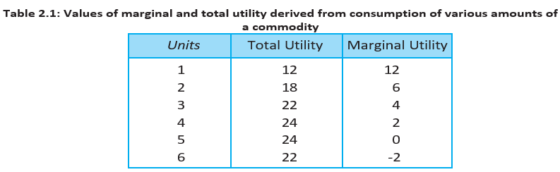
The table and graph illustrate that marginal utility decreases with each additional unit consumed, total utility increases at a diminishing rate, and eventually marginal utility can become zero or negative.

Derivation of Demand Curve Using Cardinal Utility

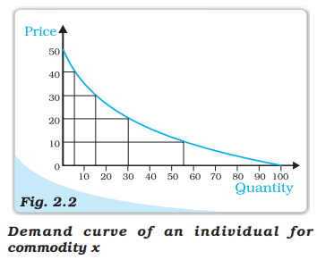
Demand is the quantity a consumer is willing and able to buy at different prices. The demand curve slopes downward due to diminishing marginal utility: as price falls, consumers buy more because the marginal utility per unit price increases.

Ordinal Utility Analysis

Ordinal utility analysis assumes consumers rank bundles by preference rather than assign numerical utility. The consumer is indifferent among bundles on the same indifference curve, which represents combinations yielding equal satisfaction.

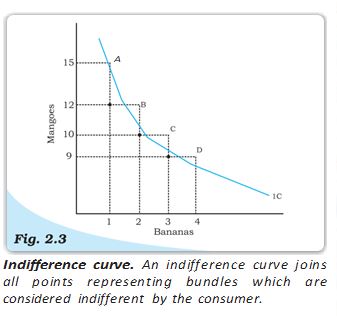
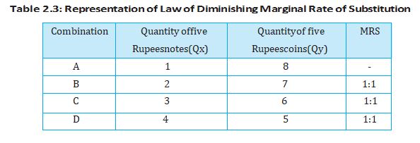
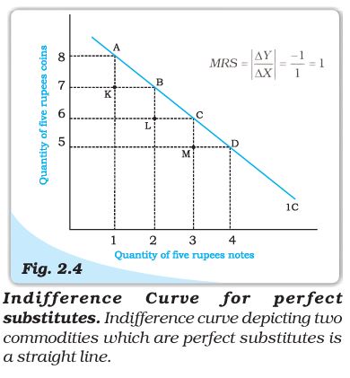
The indifference curve slopes downward because to gain more of one good, the consumer must give up some of the other to maintain the same utility level. The rate of substitution is called the Marginal Rate of Substitution (MRS):

\[ MRS = \left| \frac{\Delta Y}{\Delta X} \right| \]

where \( \Delta Y \) and \( \Delta X \) are changes in quantities of the two goods.

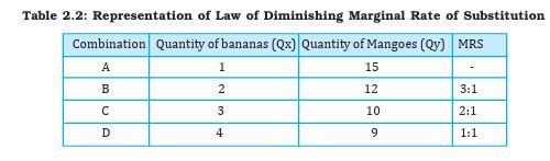
The table shows the Law of Diminishing Marginal Rate of Substitution: as the quantity of bananas increases, the consumer sacrifices fewer mangoes for each additional banana.

Indifference curves are generally convex to the origin due to diminishing MRS. For perfect substitutes, MRS is constant, and the indifference curve is a straight line.

Monotonic preferences imply that more of at least one good and no less of the other is preferred, ensuring indifference curves slope downward.

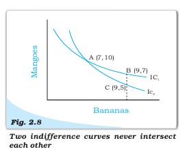
Indifference curves never intersect, as that would imply contradictory preferences.

The Consumer’s Budget

The consumer has a fixed income \( M \) and faces prices \( p_1 \) and \( p_2 \) for bananas and mangoes respectively. The consumer can afford bundles \( (x_1, x_2) \) satisfying:

\[ p_1 x_1 + p_2 x_2 \leq M \]

The set of affordable bundles is the budget set, and the budget line is where the consumer spends all income:

\[ p_1 x_1 + p_2 x_2 = M \]

The budget line intercepts are \( M/p_1 \) and \( M/p_2 \), and its slope is \( -p_1/p_2 \).

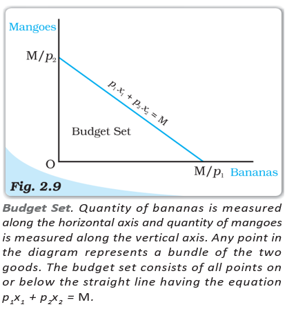
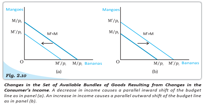
Changes in income shift the budget line parallelly; increases shift it outward, decreases inward.

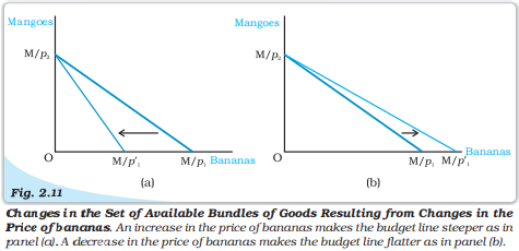
Changes in prices pivot the budget line. For example, an increase in the price of bananas makes the budget line steeper.

Optimal Choice of the Consumer

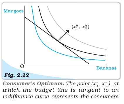
The consumer chooses the bundle that maximizes satisfaction within the budget set. The optimum is at the tangency point of the budget line and an indifference curve, where:

\[ MRS = \frac{p_1}{p_2} \]

This means the rate at which the consumer is willing to substitute goods equals the market rate of substitution.

Demand

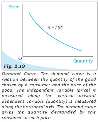
Demand is the quantity a consumer is willing and able to buy at different prices, given income and preferences. The demand function relates quantity demanded \( X \) to price \( P \):

\[ X = f(P) \]

The demand curve is generally downward sloping, reflecting the inverse relationship between price and quantity demanded.

Deriving Demand Curve from Indifference Curves and Budget Constraints

As price changes, the consumer's optimal bundle changes, tracing out the demand curve.

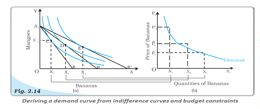
The demand curve slopes downward due to substitution and income effects when price changes.

Law of Demand

Other things being equal, demand for a commodity falls when its price rises and rises when its price falls.

Linear Demand Curve

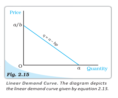
A linear demand curve can be expressed as:

\[ d(p) = a - b p \]

where \( a \) is the intercept and \( -b \) is the slope.

Normal and Inferior Goods

Demand for normal goods increases with income, while demand for inferior goods decreases with income.

Substitutes and Complements

Demand for a good increases with the price of its substitute and decreases with the price of its complement.

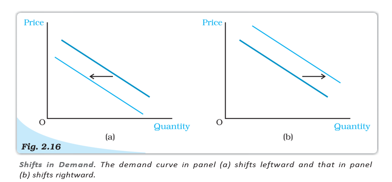
Shifts in Demand Curve

Changes in income, prices of related goods, or preferences shift the demand curve rightward (increase) or leftward (decrease).

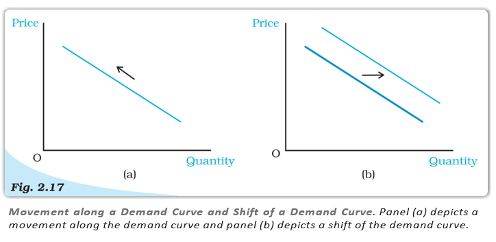
Movements Along vs Shifts of Demand Curve

Price changes cause movements along the demand curve; other factors cause shifts.

Market Demand

Market demand is the sum of individual demands at each price, obtained by horizontal summation of individual demand curves.

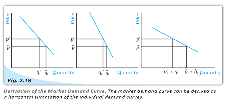
Example: If individual demands are \( d_1(p) = 10 - p \) and \( d_2(p) = 15 - p \), market demand is:

\[ d(p) = \begin{cases} 25 - 2p & p \leq 10 \\ 15 - p & 10 < p \leq 15 \\ 0 & p > 15 \end{cases} \]

Elasticity of Demand

Price elasticity of demand measures responsiveness of demand to price changes:

\[ e_D = \frac{\% \text{change in quantity demanded}}{\% \text{change in price}} = \frac{\Delta Q / Q}{\Delta P / P} = \frac{\Delta Q}{\Delta P} \times \frac{P}{Q} \]

Example: Price rises from Rs. 5 to Rs. 7, quantity demanded falls from 15 to 12 bananas.

Percentage change in quantity = \( \frac{12 - 15}{15} \times 100 = -20\% \)

Percentage change in price = \( \frac{7 - 5}{5} \times 100 = 40\% \)

Elasticity = \( \frac{20}{40} = 0.5 \) (inelastic demand)

Elasticity Along a Linear Demand Curve

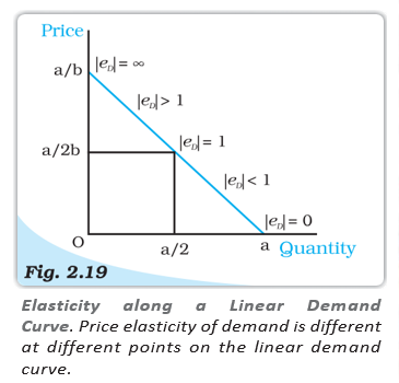
Elasticity varies along a linear demand curve:

\[ e_D = -b \times \frac{p}{a - b p} \]

At price zero, elasticity is zero; at quantity zero, elasticity is infinite; at midpoint, elasticity is one.

Geometric Measure of Elasticity

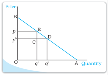
Elasticity at a point on a linear demand curve equals the ratio of the lower segment to the upper segment of the curve at that point.

Constant Elasticity Demand Curves

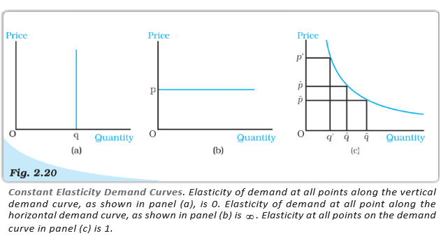
Special cases include:

• Perfectly inelastic demand (vertical curve, elasticity = 0)
• Perfectly elastic demand (horizontal curve, elasticity = infinity)
• Unitary elastic demand (rectangular hyperbola, elasticity = 1 everywhere)

Factors Determining Price Elasticity

Elasticity depends on the nature of the good and availability of substitutes. Necessities tend to have inelastic demand; luxuries and goods with close substitutes tend to have elastic demand.

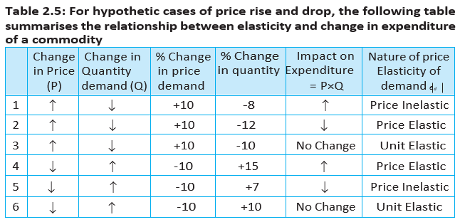
Elasticity and Expenditure

Expenditure on a good is price times quantity. Changes in expenditure due to price changes depend on elasticity:

• If demand is elastic (|e_D| > 1), expenditure moves opposite to price change.
• If demand is inelastic (|e_D| < 1), expenditure moves in the same direction as price change.
• If demand is unit elastic (|e_D| = 1), expenditure remains unchanged.

Summary

• The budget set includes all bundles affordable to the consumer; the budget line represents spending entire income.
• Consumer preferences are monotonic and can be represented by indifference curves and maps.
• Consumer's optimum is at the tangency of budget line and indifference curve.
• Demand curve shows quantity demanded at different prices, generally downward sloping.
• Normal goods have demand increasing with income; inferior goods have demand decreasing with income.
• Market demand is the sum of individual demands.
• Price elasticity of demand measures responsiveness of demand to price changes and affects expenditure.

Glossary

• Utility: Satisfaction derived from consuming goods.
• Total Utility (TU): Total satisfaction from consuming a quantity of a good.
• Marginal Utility (MU): Additional satisfaction from consuming one more unit.
• Indifference Curve: Curve showing bundles with equal satisfaction.
• Marginal Rate of Substitution (MRS): Rate at which consumer substitutes one good for another keeping utility constant.
• Budget Line: Line representing all bundles affordable with entire income spent.
• Demand Curve: Graph showing quantity demanded at different prices.
• Price Elasticity of Demand: Measure of responsiveness of demand to price changes.
• Normal Good: Demand increases with income.
• Inferior Good: Demand decreases with income.
• Substitutes: Goods that can replace each other.
• Complements: Goods consumed together.