Fundamentals and Applications of Differential Calculus
Understanding the Basics of Differentiation
Core Principles of Differential Calculus
Differential calculus focuses on determining how a function changes as its input varies. It involves calculating the derivative, which represents the instantaneous rate of change of a dependent variable with respect to an independent variable. This process, known as differentiation, can be visualized as slicing a curve into infinitesimally small segments to analyze its behavior.
When an equation expresses the derivative of a dependent variable \( y \) with respect to an independent variable \( x \), it forms a differential equation, typically written as:
\[ \frac{dy}{dx} = f(x) \]
Here, \( x \) is the independent variable, and \( y \) depends on \( x \).
Derivatives serve multiple purposes, including:
Calculating how quantities change over time or other variables.
Deriving equations for tangents and normals to curves at specific points.
Identifying turning points to find local maxima and minima on graphs.
Determining intervals where functions increase or decrease.
Estimating approximate values of functions near known points.
Illustrative Problem
Calculate the rate at which the area of a circle changes with respect to its radius when the radius is 7 cm.
Solution:
The area \( A \) of a circle is given by:
\[ A = \pi r^2 \]
To find the rate of change of area with respect to radius, differentiate \( A \) with respect to \( r \):
\[ \frac{dA}{dr} = \frac{d}{dr} (\pi r^2) = 2 \pi r \]
Substituting \( r = 7 \text{ cm} \):
\[ \frac{dA}{dr} = 2 \pi \times 7 = 14 \pi \text{ cm}^2/\text{s} \]
Thus, the area increases at a rate of \( 14 \pi \text{ cm}^2/\text{s} \) when the radius is 7 cm.
Approximating Changes Using Differentials
Conceptualizing Differentials for Estimation
Differentials provide a method to approximate small changes in function values based on small changes in the input variable. Consider a function \( y = f(x) \) defined on a domain \( D \subset \mathbb{R} \). If the input \( x \) increases by a small amount \( \Delta x \), the corresponding change in \( y \) is:
\[ \Delta y = f(x + \Delta x) - f(x) \]
The differential of \( x \), denoted \( dx \), is defined as \( dx = \Delta x \). The differential of \( y \), denoted \( dy \), is given by:
\[ dy = f'(x) dx = \frac{dy}{dx} \Delta x \]
When \( \Delta x \) is very small, \( dy \) closely approximates \( \Delta y \), so \( dy \approx \Delta y \). This approximation is useful for estimating function values near known points.
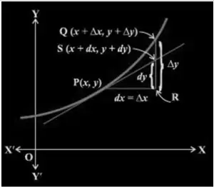
This is often used when learning about derivatives in calculus.
Graph illustrating the relationship between \( \Delta x \), \( \Delta y \), and differentials
Example 1: Estimating Square Root Using Differentials
Approximate \( \sqrt{16.3} \) using the concept of differentials.
Solution:
Let \( y = \sqrt{x} \), with \( x = 16 \) and \( \Delta x = 0.3 \).
The change in \( y \) is:
\[ \Delta y = \sqrt{16.3} - \sqrt{16} = \sqrt{16.3} - 4 \]
Since \( dy \approx \Delta y \), calculate \( dy \):
\[ dy = \frac{dy}{dx} \Delta x = \frac{1}{2 \sqrt{x}} \times \Delta x = \frac{1}{2 \times 4} \times 0.3 = 0.0375 \]
Therefore, the approximate value is:
\[ \sqrt{16.3} \approx 4 + 0.0375 = 4.0375 \]
Example 2: Approximating a Polynomial Function Value
Estimate \( f(2.05) \) for the function \( f(x) = 4x^2 + 3x + 1 \).
Solution:
Given \( f(x) = 4x^2 + 3x + 1 \), let \( x = 2 \) and \( \Delta x = 0.05 \).
Calculate the derivative:
\[ f'(x) = 8x + 3 \]
Using the differential approximation:
\[ f(2.05) \approx f(2) + f'(2) \Delta x \]
Calculate each term:
\[ f(2) = 4(2)^2 + 3(2) + 1 = 16 + 6 + 1 = 23 \]
\[ f'(2) = 8(2) + 3 = 16 + 3 = 19 \]
Therefore:
\[ f(2.05) \approx 23 + 19 \times 0.05 = 23 + 0.95 = 23.95 \]
Practical Applications and Problem Solving with Differentials
Utilizing Differentials for Error Estimation and Approximations
Differentials are valuable tools for estimating errors in measurements and approximating function values when exact calculations are complex. They help in predicting how small changes in input affect the output, which is essential in fields like physics, engineering, and economics.
Example 3: Estimating Error in Surface Area Measurement
A sphere has a radius measured as 10 cm with a possible error of 0.04 cm. Estimate the maximum error in the calculated surface area.
Solution:
The surface area \( S \) of a sphere is:
\[ S = 4 \pi r^2 \]
The differential \( dS \) approximates the error in surface area:
\[ dS = \frac{dS}{dr} dr = 8 \pi r \, dr \]
Substitute \( r = 10 \text{ cm} \) and \( dr = 0.04 \text{ cm} \):
\[ dS = 8 \pi \times 10 \times 0.04 = 3.2 \pi \text{ cm}^2 \]
Thus, the surface area may have an error of approximately \( 3.2 \pi \text{ cm}^2 \).
Exam Tip: When using differentials for approximations, always identify the independent variable and calculate the derivative correctly before substituting values.
Quick Reference: Key Formulas and Concepts
Concept | Formula/Definition | Usage |
|---|---|---|
Derivative | \( \frac{dy}{dx} = f'(x) \) | Rate of change of \( y \) with respect to \( x \) |
Differential of \( x \) | \( dx = \Delta x \) | Small change in independent variable |
Differential of \( y \) | \( dy = f'(x) dx \) | Approximate change in dependent variable |
Area of Circle | \( A = \pi r^2 \) | Calculate area based on radius |
Rate of change of area | \( \frac{dA}{dr} = 2 \pi r \) | How area changes with radius |
Surface Area of Sphere | \( S = 4 \pi r^2 \) | Calculate surface area from radius |
Error in Surface Area | \( dS = 8 \pi r \, dr \) | Estimate error from radius measurement |
Approximate function value | \( f(x + \Delta x) \approx f(x) + f'(x) \Delta x \) | Estimate function near \( x \) |
Turning Points | \( f'(x) = 0 \) | Find maxima or minima of function |
Equation of Tangent | \( y - y_1 = f'(x_1)(x - x_1) \) | Line touching curve at one point |
Glossary of Important Terms
Term | Meaning |
|---|---|
Derivative | The instantaneous rate of change of a function with respect to a variable. |
Differential | An infinitesimally small change in a variable, used for approximations. |
Independent Variable | The variable with respect to which differentiation is performed. |
Dependent Variable | The variable whose value depends on the independent variable. |
Differential Equation | An equation involving derivatives of a function. |
Turning Point | A point on a curve where the function changes from increasing to decreasing or vice versa. |
Tangent | A straight line that touches a curve at a point without crossing it. |
Normal | A line perpendicular to the tangent at the point of contact on a curve. |
Approximation | Estimating a value close to the actual value using differentials. |
Rate of Change | The speed at which one quantity changes relative to another. |
Frequently Asked Questions
What is the main purpose of differentiation?
Differentiation helps find how a function changes at any point, providing the rate of change of one variable with respect to another.
How do differentials help in approximations?
Differentials estimate small changes in function values based on small changes in input, allowing approximate calculations near known points.
What is the difference between \( dy \) and \( \Delta y \)?
\( dy \) is the differential representing an approximate change, while \( \Delta y \) is the actual change in the function value.
How can derivatives be used to find turning points?
Turning points occur where the derivative equals zero, indicating potential maxima or minima of the function.
Why is the derivative of the area of a circle with respect to radius important?
It shows how quickly the area changes as the radius changes, useful in problems involving growth or measurement errors.