Damped Oscillations: Understanding Energy Loss in Harmonic Systems
Fundamentals of Energy Dissipation in Oscillatory Motion
Nature and Causes of Damping in Oscillators
Ideal harmonic oscillators maintain constant total energy, resulting in perpetual oscillations with fixed amplitude and frequency determined by the system's inertia and elasticity. Such idealized motions are termed free or undamped oscillations.
In reality, oscillations gradually lose energy due to resistive forces like friction and air resistance, causing the amplitude to diminish over time until the motion ceases. For instance, a pendulum swinging in air slows down and eventually stops, and the vibrations of a tuning fork fade away.
Damping forces oppose the motion, performing negative work and converting mechanical energy into heat within the system or its surroundings. Additionally, oscillators lose energy by radiating waves, such as sound waves produced by a tuning fork, which carry energy away from the system.
Consequently, the amplitude reduction over time is known as damping, and the resulting motion is called damped oscillation.
Example: A pendulum oscillating in air experiences a gradual decrease in amplitude due to air resistance and friction at the pivot, illustrating damping in a real system.
Types and Characteristics of Damping Forces
Classification and Mathematical Description of Damping
Damping arises from various forces that resist motion. The most common is viscous damping, where the damping force is proportional to the velocity and acts opposite to it. This force can be expressed as \( F_d = -p v \), where \( p \) is the viscous damping coefficient and \( v \) is the velocity magnitude.
Other damping types include Coulomb friction, a constant magnitude force opposing motion, often encountered when oscillating parts contact unlubricated surfaces, and structural damping, caused by internal friction within materials, typically proportional to amplitude but independent of frequency.
Due to the complexity of real damping, viscous damping is often used as an approximation for mathematical convenience, with the coefficient chosen to match the actual energy dissipation rate.
Example: In a spring-mass system oscillating horizontally on a rough surface, the frictional force opposing motion can be modeled as Coulomb friction, a constant force resisting the movement.
Mathematical Modeling of Damped Oscillations
Deriving the Equation of Motion for a Damped Oscillator
Consider a single degree of freedom system with mass \( m \), subjected to a restoring force proportional to displacement \( -Kx \) and a damping force proportional to velocity \( -p \frac{dx}{dt} \). Applying Newton's second law yields:
\[ m \frac{d^2 x}{dt^2} = -p \frac{dx}{dt} - K x \]
Rearranged, the equation becomes:
\[ \frac{d^2 x}{dt^2} + \gamma \frac{dx}{dt} + \omega_0^2 x = 0 \]
where \( \gamma = \frac{p}{m} \) is the damping factor with units of inverse time, and \( \omega_0 = \sqrt{\frac{K}{m}} \) is the natural angular frequency of the undamped system.
Example: For a mass of 2 kg attached to a spring with spring constant 50 N/m and damping coefficient 4 Ns/m, calculate \( \gamma \) and \( \omega_0 \):
\[ \gamma = \frac{4}{2} = 2 \text{ s}^{-1}, \quad \omega_0 = \sqrt{\frac{50}{2}} = 5 \text{ rad/s} \]
Solutions and Behavior of Damped Oscillators
General Solution and Classification Based on Damping Magnitude
The characteristic equation associated with the damped oscillator is:
\[ \alpha^2 + \gamma \alpha + \omega_0^2 = 0 \]
Its roots determine the system's response:
Overdamped (\( \gamma > 2 \omega_0 \)): Two distinct real roots lead to non-oscillatory motion where displacement returns to equilibrium without crossing zero.
Critically damped (\( \gamma = 2 \omega_0 \)): Repeated real root causes the system to return to equilibrium as quickly as possible without oscillating.
Underdamped (\( \gamma < 2 \omega_0 \)): Complex conjugate roots produce oscillatory motion with exponentially decaying amplitude.
Example: For a system with \( \gamma = 6 \text{ s}^{-1} \) and \( \omega_0 = 2 \text{ rad/s} \), determine the damping case:
Since \( 2 \omega_0 = 4 \text{ s}^{-1} \) and \( \gamma = 6 > 4 \), the system is overdamped.
Detailed Analysis of Overdamped Motion
Behavior and Mathematical Formulation of Heavy Damping
In the overdamped regime, the displacement is expressed as:
\[ x(t) = A_1 e^{\alpha_1 t} + A_2 e^{\alpha_2 t} \]
where \( \alpha_1 \) and \( \alpha_2 \) are negative real roots. The motion does not oscillate but slowly returns to equilibrium.
For initial conditions \( x(0) = 0 \) and initial velocity \( V_0 \), constants are:
\[ A_1 = -A_2 = \frac{V_0}{2q} \]
with \( q = \sqrt{\frac{\gamma^2}{4} - \omega_0^2} \).
The displacement simplifies to:
\[ x(t) = \frac{V_0}{q} e^{-\frac{\gamma t}{2}} \sinh(q t) \]
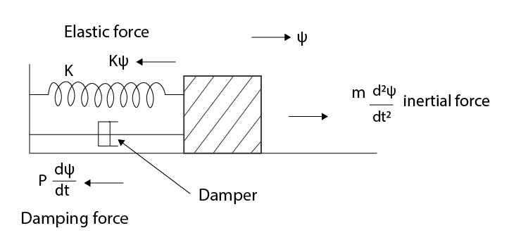
Figure 1: Displacement-time graph of a heavily damped oscillator
Example: A damped oscillator with \( \gamma = 6 \text{ s}^{-1} \), \( \omega_0 = 2 \text{ rad/s} \), and initial velocity \( V_0 = 3 \text{ m/s} \) has \( q = \sqrt{9 - 4} = \sqrt{5} \approx 2.236 \text{ s}^{-1} \). The displacement at \( t = 1 \text{ s} \) is:
\[ x(1) = \frac{3}{2.236} e^{-3} \sinh(2.236) \approx 1.342 \times 0.0498 \times 4.81 \approx 0.32 \text{ m} \]
Critical Damping: Fastest Return Without Oscillation
Mathematical Solution and Physical Significance
When \( \gamma = 2 \omega_0 \), the system is critically damped. The general solution is:
\[ x(t) = (B + C t) e^{-\frac{\gamma t}{2}} \]
Applying initial conditions \( x(0) = 0 \) and \( \frac{dx}{dt}(0) = V_0 \) yields:
\[ B = 0, \quad C = V_0 \]
Thus, displacement becomes:
\[ x(t) = V_0 t e^{-\frac{\gamma t}{2}} \]
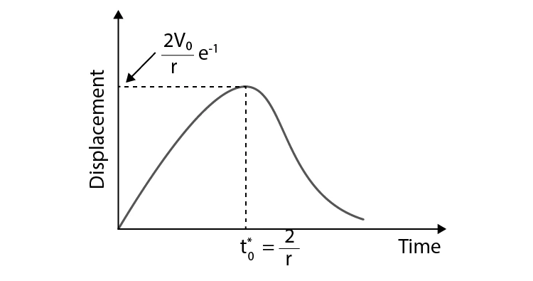
Figure 2: Displacement-time graph of a critically damped oscillator
Example: For a system with \( \gamma = 4 \text{ s}^{-1} \) and initial velocity \( V_0 = 2 \text{ m/s} \), find displacement at \( t = 0.5 \text{ s} \):
\[ x(0.5) = 2 \times 0.5 \times e^{-2 \times 0.5} = 1 \times e^{-1} \approx 0.368 \text{ m} \]
Oscillatory Motion in Weakly Damped Systems
Solution and Characteristics of Underdamped Oscillations
For \( \gamma < 2 \omega_0 \), the roots are complex conjugates, and the displacement is:
\[ x(t) = A e^{-\frac{\gamma t}{2}} \cos(\omega^* t - \delta) \]
where the damped angular frequency is:
\[ \omega^* = \omega_0 \sqrt{1 - \frac{\gamma^2}{4 \omega_0^2}} \]
Constants \( A \) and \( \delta \) depend on initial conditions. For \( x(0) = 0 \) and \( \frac{dx}{dt}(0) = V_0 \), we find:
\[ \delta = \frac{\pi}{2}, \quad A = \frac{V_0}{\omega^*} \]
Hence, displacement and velocity are:
\[ x(t) = \frac{V_0}{\omega^*} e^{-\frac{\gamma t}{2}} \sin(\omega^* t) \]
\[ \frac{dx}{dt} = V_0 e^{-\frac{\gamma t}{2}} \left( \cos(\omega^* t) - \frac{\gamma}{2 \omega^*} \sin(\omega^* t) \right) \]
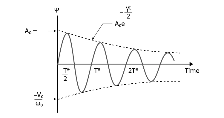
Figure 3: Displacement-time graph of a weakly damped oscillator
Example: A system with \( \omega_0 = 10 \text{ rad/s} \), \( \gamma = 1 \text{ s}^{-1} \), and initial velocity \( V_0 = 5 \text{ m/s} \) has:
\[ \omega^* = 10 \sqrt{1 - \frac{1^2}{4 \times 10^2}} \approx 9.987 \text{ rad/s} \]
Amplitude at \( t = 0 \) is \( A = \frac{5}{9.987} \approx 0.501 \text{ m} \).
Energy Dynamics in Weakly Damped Oscillators
Time Evolution of Energy and Power Dissipation
The instantaneous kinetic energy is:
\[ KE = \frac{1}{2} m \left( \frac{dx}{dt} \right)^2 = \frac{1}{2} m A^2 e^{-\gamma t} \left( \omega^* \sin(\omega^* t - \delta) + \frac{\gamma}{2} \cos(\omega^* t - \delta) \right)^2 \]
The potential energy is:
\[ PE = \frac{1}{2} K x^2 = \frac{1}{2} m \omega_0^2 A^2 e^{-\gamma t} \cos^2(\omega^* t - \delta) \]
The total energy is the sum:
\[ E(t) = KE + PE = \frac{1}{2} m A^2 e^{-\gamma t} \left( \omega^{*2} \sin^2(\omega^* t - \delta) + \frac{\gamma \omega^*}{2} \sin 2(\omega^* t - \delta) + \left( \frac{\gamma^2}{4} + \omega_0^2 \right) \cos^2(\omega^* t - \delta) \right) \]
Assuming \( \gamma \) is small, the time-averaged energy over one period \( T^* = \frac{2\pi}{\omega^*} \) is:
\[ \langle E(t) \rangle = \frac{1}{2} m A^2 \omega_0^2 e^{-\gamma t} = E_0 e^{-\gamma t} \]
where \( E_0 \) is the initial energy of the undamped oscillator.
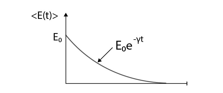
Figure 4: Exponential decay of total energy during damping
The average power dissipated is the rate of energy loss:
\[ \langle P(t) \rangle = -\frac{d}{dt} \langle E(t) \rangle = \gamma E_0 e^{-\gamma t} = \gamma \langle E(t) \rangle \]
This power loss corresponds to work done against frictional forces and energy radiated away as waves.
Example: For a damped oscillator with initial energy \( E_0 = 10 \text{ J} \) and damping factor \( \gamma = 0.1 \text{ s}^{-1} \), the energy after 5 seconds is:
\[ \langle E(5) \rangle = 10 e^{-0.1 \times 5} = 10 e^{-0.5} \approx 6.07 \text{ J} \]
Summary of Key Concepts in Damped Oscillations
Concept | Description | Mathematical Expression |
|---|---|---|
Damping Force | Opposes motion, proportional to velocity | \( F_d = -p v \) |
Damping Factor | Ratio of damping coefficient to mass | \( \gamma = \frac{p}{m} \) |
Natural Frequency | Frequency without damping | \( \omega_0 = \sqrt{\frac{K}{m}} \) |
Damped Frequency | Frequency with damping | \( \omega^* = \omega_0 \sqrt{1 - \frac{\gamma^2}{4 \omega_0^2}} \) |
Energy Decay | Exponential decrease of total energy | \( E(t) = E_0 e^{-\gamma t} \) |
Oscillation Types | Overdamped, critically damped, underdamped | Based on relation between \( \gamma \) and \( 2 \omega_0 \) |
Equation of Motion | Damped harmonic oscillator differential equation | \( \frac{d^2 x}{dt^2} + \gamma \frac{dx}{dt} + \omega_0^2 x = 0 \) |
Power Dissipation | Rate of energy loss due to damping | \( \langle P(t) \rangle = \gamma \langle E(t) \rangle \) |
Critical Damping Condition | Fastest return to equilibrium without oscillation | \( \gamma = 2 \omega_0 \) |
Overdamped Motion | Non-oscillatory return to equilibrium | Two distinct negative real roots of characteristic equation |
Glossary of Terms Related to Damped Oscillations
Term | Definition |
|---|---|
Damping | Reduction in amplitude of oscillations due to resistive forces |
Viscous Damping | Damping force proportional to velocity |
Coulomb Friction | Constant magnitude friction force opposing motion |
Structural Damping | Energy loss due to internal friction in materials |
Natural Frequency (\( \omega_0 \)) | Frequency of undamped oscillations |
Damped Frequency (\( \omega^* \)) | Frequency of oscillations with damping |
Overdamped | Damping greater than critical, no oscillations |
Critically Damped | Minimum damping to prevent oscillations |
Underdamped | Damping less than critical, oscillations with decaying amplitude |
Energy Dissipation | Conversion of mechanical energy into heat or radiation |
Frequently Asked Questions on Damped Oscillations
What defines a damped oscillation?
Damped oscillations are periodic motions where the amplitude decreases over time due to resistive forces like friction or air resistance.
How does an undamped oscillation differ?
Undamped oscillations maintain constant amplitude indefinitely, as no energy is lost from the system.
What are common examples of damped oscillations?
Examples include the swinging of a pendulum in air and the vibrations of a swing gradually slowing down.
What is critical damping and why is it important?
Critical damping is the exact amount of damping that allows the system to return to equilibrium as quickly as possible without oscillating, useful in devices like galvanometers.
How does damping affect the frequency of oscillations?
Damping reduces the oscillation frequency slightly below the natural frequency, with the damped frequency given by \( \omega^* = \omega_0 \sqrt{1 - \frac{\gamma^2}{4 \omega_0^2}} \).