Understanding Continuous Charge Distributions and Electric Field Calculations
Concept of Continuous Charge Distribution
Defining Charge Density for Various Distributions
In many practical scenarios, charges are not isolated points but spread continuously over a region. Instead of treating each charge separately, we consider the charge spread over a length, surface, or volume. This approach simplifies calculations by introducing the concept of charge density, which quantifies how much charge exists per unit length, area, or volume.
For example, when charges are spread over a surface, we define the surface charge density \( \sigma \) as the charge per unit area. If a small surface element \( \Delta s \) carries a charge \( \Delta Q \), then
\[ \sigma = \frac{\Delta Q}{\Delta s} \]
The SI unit of surface charge density is Coulombs per square meter (\(\text{C/m}^2\)).
Similarly, for charges distributed along a thin wire or line segment of length \( \Delta l \), the linear charge density \( \lambda \) is defined as
\[ \lambda = \frac{\Delta Q}{\Delta l} \]
with units Coulombs per meter (\(\text{C/m}\)).
When charges occupy a volume element \( \Delta V \), the volume charge density \( \rho \) is given by
\[ \rho = \frac{\Delta Q}{\Delta V} \]
and its unit is Coulombs per cubic meter (\(\text{C/m}^3\)).
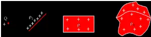
Diagram illustrating discrete point charges and continuous charge distribution
Example: Calculating Linear Charge Density
A wire of length 0.5 meters carries a total charge of \( 3.5 \times 10^{-6} \text{ C} \) uniformly distributed along its length. Determine the linear charge density \( \lambda \).
Solution:
The linear charge density is the charge per unit length:
\[ \lambda = \frac{Q}{L} = \frac{3.5 \times 10^{-6} \text{ C}}{0.5 \text{ m}} = 7.0 \times 10^{-6} \text{ C/m} \]
Thus, the wire has a linear charge density of \( 7.0 \times 10^{-6} \text{ C/m} \).
Determining Electric Field from Distributed Charges
Calculating the Field Due to Volume Charge Distribution
When charges are spread continuously in a volume, the electric field at a point due to the entire distribution can be found by summing contributions from infinitesimal volume elements. Each small volume element \( \Delta V \) with charge density \( \rho \) contains charge \( \rho \Delta V \).
If the distance from this volume element to the point of interest \( P \) is \( r \), then by Coulomb’s law, the electric field contribution \( \Delta \mathbf{E} \) from this element is
\[ \Delta \mathbf{E} = \frac{1}{4 \pi \epsilon_0} \frac{\rho \Delta V}{r^2} \hat{r} \]
where \( \hat{r} \) is the unit vector pointing from the charge element to point \( P \), and \( \epsilon_0 \) is the permittivity of free space.
To find the total electric field \( \mathbf{E} \), integrate over the entire volume:
\[ \mathbf{E} = \frac{1}{4 \pi \epsilon_0} \int \frac{\rho(\mathbf{r}')}{|\mathbf{r} - \mathbf{r}'|^2} \hat{r} \, dV' \]
This integral accounts for the vector nature of the field and the spatial variation of charge density.
Example: Electric Field from a Uniformly Charged Sphere
A solid sphere of radius 0.1 m carries a uniform volume charge density \( \rho = 5 \times 10^{-6} \text{ C/m}^3 \). Calculate the magnitude of the electric field at a point 0.15 m from the center of the sphere.
Solution:
Since the point lies outside the sphere, the entire charge can be treated as concentrated at the center.
Total charge \( Q \) is
\[ Q = \rho \times \frac{4}{3} \pi R^3 = 5 \times 10^{-6} \times \frac{4}{3} \pi (0.1)^3 = 2.09 \times 10^{-7} \text{ C} \]
Electric field at distance \( r = 0.15 \text{ m} \) is
\[ E = \frac{1}{4 \pi \epsilon_0} \frac{Q}{r^2} = 9 \times 10^9 \times \frac{2.09 \times 10^{-7}}{(0.15)^2} = 8.36 \times 10^4 \text{ N/C} \]
Therefore, the electric field magnitude at 0.15 m from the center is \( 8.36 \times 10^4 \text{ N/C} \).
Types of Continuous Charge Distributions and Their Applications
Exploring Linear, Surface, and Volume Charge Densities
Continuous charge distributions are categorized based on the dimension over which the charge is spread:
Linear charge distribution: Charge spread along a line, characterized by linear charge density \( \lambda \).
Surface charge distribution: Charge spread over a surface area, described by surface charge density \( \sigma \).
Volume charge distribution: Charge distributed throughout a volume, quantified by volume charge density \( \rho \).
Each type requires different integration methods to calculate electric fields or potentials, depending on the geometry and symmetry.
Example: Surface Charge Density on a Charged Plate
A square metal plate of side 0.2 m carries a total charge of \( 1.2 \times 10^{-5} \text{ C} \) uniformly distributed over its surface. Find the surface charge density \( \sigma \).
Solution:
Area of the plate is
\[ A = (0.2 \text{ m})^2 = 0.04 \text{ m}^2 \]
Surface charge density is
\[ \sigma = \frac{Q}{A} = \frac{1.2 \times 10^{-5} \text{ C}}{0.04 \text{ m}^2} = 3.0 \times 10^{-4} \text{ C/m}^2 \]
Hence, the surface charge density on the plate is \( 3.0 \times 10^{-4} \text{ C/m}^2 \).
Summary of Key Concepts
Charge Distribution Type | Charge Density Symbol | Definition | SI Unit |
|---|---|---|---|
Linear | \( \lambda \) | Charge per unit length | Coulombs per meter (C/m) |
Surface | \( \sigma \) | Charge per unit area | Coulombs per square meter (C/m²) |
Volume | \( \rho \) | Charge per unit volume | Coulombs per cubic meter (C/m³) |
Electric Field from Volume Charge | – | \( \mathbf{E} = \frac{1}{4 \pi \epsilon_0} \int \frac{\rho}{r^2} \hat{r} \, dV \) | Newtons per Coulomb (N/C) |
Glossary of Important Terms
Term | Meaning |
|---|---|
Charge Density | Amount of electric charge per unit length, area, or volume |
Linear Charge Density (\( \lambda \)) | Charge per unit length along a line |
Surface Charge Density (\( \sigma \)) | Charge per unit area on a surface |
Volume Charge Density (\( \rho \)) | Charge per unit volume within a body |
Coulomb’s Law | Law describing the force between two point charges |
Electric Field (\( \mathbf{E} \)) | Force per unit charge experienced by a test charge |
Permittivity of Free Space (\( \epsilon_0 \)) | Constant defining electric field behavior in vacuum |
Superposition Principle | Electric fields from multiple charges add vectorially |
Unit Vector (\( \hat{r} \)) | Vector indicating direction from charge to point of interest |
Continuous Charge Distribution | Charge spread smoothly over a region rather than discrete points |
Frequently Asked Questions
What is meant by continuous charge distribution?
It refers to charges spread smoothly over a length, surface, or volume, rather than existing as isolated point charges.
How is surface charge density defined?
Surface charge density \( \sigma \) is the amount of charge per unit area on a surface, measured in Coulombs per square meter.
Why do we use charge density instead of discrete charges?
When charges are too numerous or closely packed, treating them as continuous distributions simplifies calculations and models physical reality better.
How is the electric field calculated from a volume charge distribution?
By integrating the contributions of infinitesimal volume elements, each producing a small electric field, over the entire charged volume.
What is the significance of the unit vector \( \hat{r} \) in electric field calculations?
It indicates the direction from the charge element to the point where the field is being calculated, ensuring the vector nature of the field is accounted for.