Understanding Cumulative Frequency Distribution and Its Applications
Fundamentals of Cumulative Frequency Distribution
Concept and Purpose of Cumulative Frequency
Cumulative frequency represents the running total of frequencies across successive class intervals in a data set. Starting from the first class, each frequency is added to the sum of all previous frequencies, creating a cumulative total that increases as we move through the classes. This approach helps in understanding how data accumulates over intervals and is essential for analyzing the distribution of observations below or above certain values.
By organizing data into a cumulative frequency table, statisticians can easily identify the number of observations that fall within or beyond specific ranges, facilitating deeper insights into the data's behavior.
\[ 5 + 8 + 12 = 25 \]
Classification of Cumulative Frequency Types
Less Than Cumulative Frequency Explained
The "less than" cumulative frequency is obtained by successively adding the frequencies starting from the lowest class interval up to the current class. This method accumulates frequencies from the smallest values upwards, providing a cumulative count of observations less than or equal to the upper boundary of each class.
This type is particularly useful for determining the proportion of data below a certain threshold and is commonly used in constructing ogive curves.
\[ 4 + 7 + 9 = 20 \]
This means 20 observations fall below or within the 30-40 class interval.More Than Cumulative Frequency Overview
The "more than" cumulative frequency is calculated by adding frequencies starting from the highest class interval down to the current class. This approach accumulates frequencies from the largest values downwards, showing the total number of observations greater than or equal to the lower boundary of each class.
This type is valuable for analyzing data above certain limits and is also used in plotting ogive curves.
\[ 8 + 6 = 14 \]
This indicates 14 observations are greater than or equal to 40.Graphical Interpretation and Median Determination
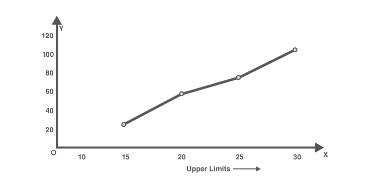
Constructing the Less Than Cumulative Frequency Curve
To plot the less than cumulative frequency curve (ogive), follow these steps:
- Label the x-axis with the upper class boundaries.
- Label the y-axis with cumulative frequencies.
- Plot points where the x-coordinate is the upper class limit and the y-coordinate is the corresponding cumulative frequency.
- Connect the points smoothly to form the curve.
This curve visually represents the accumulation of data up to each class limit.
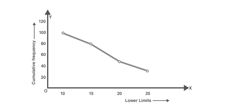
Steps to Draw the More Than Cumulative Frequency Curve
For the more than cumulative frequency curve, the procedure is:
- Mark the lower class boundaries on the x-axis.
- Mark cumulative frequencies on the y-axis.
- Plot points with x as the lower class limit and y as the cumulative frequency.
- Join the points with a smooth curve.
This curve shows the accumulation of data from the highest values downwards.
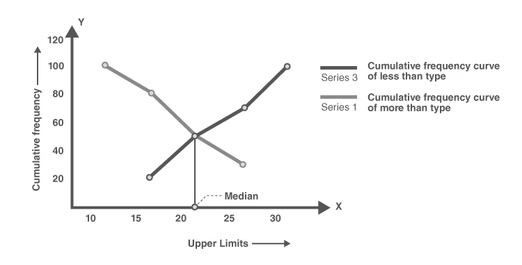
The intersection point of these two curves corresponds to the median of the data set, providing a graphical method to estimate the median value.
Practical Application: Creating a Cumulative Frequency Table
Example: Weekly Indoor Game Hours of a Student
Consider Arjun's weekly indoor game hours recorded as follows:
| Hours Played (Class Interval) | Number of Days (Frequency) |
|---|---|
| 0-2 | 3 |
| 2-4 | 5 |
| 4-6 | 7 |
| 6-8 | 4 |
| 8-10 | 1 |
To find the cumulative frequency, add the frequencies successively:
| Hours Played (Class Interval) | Frequency | Cumulative Frequency |
|---|---|---|
| 0-2 | 3 | 3 |
| 2-4 | 5 | 8 |
| 4-6 | 7 | 15 |
| 6-8 | 4 | 19 |
| 8-10 | 1 | 20 |
Thus, Arjun spends a total of 20 hours per week playing indoor games.
- Start with the first frequency: 3.
- Add the second frequency: \(3 + 5 = 8\).
- Add the third frequency: \(8 + 7 = 15\).
- Add the fourth frequency: \(15 + 4 = 19\).
- Add the fifth frequency: \(19 + 1 = 20\).
Therefore, the cumulative frequency column is: 3, 8, 15, 19, 20.
Quick Reference: Key Points on Cumulative Frequency
| Concept | Explanation |
|---|---|
| Cumulative Frequency | Running total of frequencies up to a class interval. |
| Less Than Type | Sum of frequencies from the lowest class up to the current class. |
| More Than Type | Sum of frequencies from the highest class down to the current class. |
| Ogive | Graphical representation of cumulative frequency distribution. |
| Median from Ogives | Point where less than and more than ogives intersect. |
| Class Interval | Range of values grouped together in frequency distribution. |
| Frequency | Number of observations in a class interval. |
| Cumulative Frequency Table | Table showing cumulative frequencies for each class interval. |
| Upper Class Boundary | Highest value included in a class interval. |
| Lower Class Boundary | Lowest value included in a class interval. |
Glossary of Important Terms
| Term | Definition |
|---|---|
| Cumulative Frequency | The total frequency accumulated up to a certain class interval. |
| Class Interval | A range of values grouped together in a frequency distribution. |
| Frequency | The count of observations within a class interval. |
| Less Than Ogive | A curve representing cumulative frequencies up to upper class limits. |
| More Than Ogive | A curve representing cumulative frequencies from lower class limits downwards. |
| Median | The middle value of a data set when arranged in order. |
| Upper Class Boundary | The maximum value included in a class interval. |
| Lower Class Boundary | The minimum value included in a class interval. |
| Ogive | A graph showing cumulative frequency distribution. |
| Data Set | A collection of observations or values. |
Frequently Asked Questions
What does cumulative frequency represent?
Cumulative frequency is the total count of observations accumulated up to a specific class interval in a data set.
How is a cumulative frequency distribution table constructed?
By successively adding the frequencies of each class interval to the sum of all previous frequencies, forming a running total.
What are the two main types of cumulative frequency?
They are the less than cumulative frequency, which accumulates from the lowest class upwards, and the more than cumulative frequency, which accumulates from the highest class downwards.
How can the median be found using cumulative frequency curves?
The median corresponds to the point where the less than and more than cumulative frequency curves intersect on a graph.
Why is cumulative frequency useful in data analysis?
It helps in understanding the distribution of data, identifying medians, percentiles, and making comparisons between different data sets.